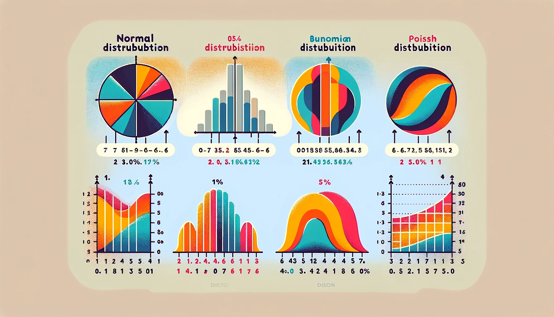
Statistical Distributions

Statistical distributions are fundamental in understanding and representing how data values are spread or varied. Each distribution has its own unique properties and applications. The type of statistical distribution used often depends on the type of variable (continuous and discrete)

Discrete Variables

Bernoulli Distribution

The Bernoulli distribution is a simple discrete probability distribution that has only two possible outcomes, commonly labeled as “success” and “failure.” The number of trials is just one (a special case of the binomial distribution).

Key aspects The probability mass function (PMF) of a Bernoulli distribution is given by:

$\begin{cases} p & \text{if } k=1, \\ 1-p & \text{if } k=0 \end{cases}$

Examples:

• Flipping a coin (where heads could be defined as success and tails as failure).
• A quality control check where an item is either defective (failure) or non-defective (success).

Python Example: To simulate a Bernoulli trial using we could use numpy.random.binomial with n=1.

# Parameters for Bernoulli distribution
p = 0.5  # Probability of success
size = 1000  # Number of samples

# Generating Bernoulli samples
bernoulli_samples = np.random.binomial(1, p, size) # it generates either 1 or 0 'size' times.

# Plotting the distribution
plt.figure(figsize=(6, 4))
plt.hist(bernoulli_samples, bins=[-0.5, 0.5, 1.5], rwidth=0.5, color='blue', alpha=0.7)
plt.xticks([0, 1])
plt.title('Bernoulli Distribution (p = 0.5)')
plt.xlabel('Outcome')
plt.ylabel('Frequency')
plt.show()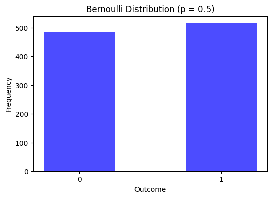

Binomial Distribution

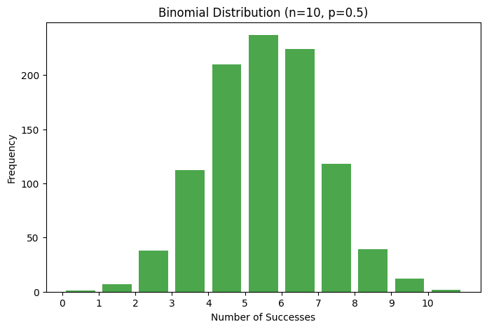
The Binomial distribution is a discrete probability distribution that describes the number of successes in a fixed number of independent trials of a binary experiment. It is an extension of the Bernoulli distribution across multiple trials.

Probability math representation: $P(X = k) = (\frac{n}{k})p^k(1-p)^{n-k}$

where $(\frac{n}{k})$ is the binomial coefficient, $n$ is number of trials, $k$ is the number of successes, and $p$ the probability of success.

Examples:

• Flipping a coin a certain number of times and counting the number of heads (or tails).
• The number of defective items in a batch when each item has a fixed probability of being defective.

Python Example: The Binomial distribution can be simulated using numpy.random.binomial(n, p, size), where n is the number of trials, p is the probability of success, and size is the number of experiments.

# Parameters for Binomial distribution
n = 10  # Number of trials
p = 0.5  # Probability of success
size = 1000  # Number of samples

# Generating Binomial samples
binomial_samples = np.random.binomial(n, p, size)

# Plotting the distribution
plt.figure(figsize=(8, 5))
plt.hist(binomial_samples, bins=range(n+2), rwidth=0.8, color='green', alpha=0.7)
plt.title('Binomial Distribution (n=10, p=0.5)')
plt.xlabel('Number of Successes')
plt.ylabel('Frequency')
plt.xticks(range(n+1))
plt.show()

Poisson Distribution

The Poisson distribution is a discrete probability distribution that expresses the probability of a given number of events occurring in a fixed interval of time or space, assuming these events occur with a known constant mean rate and independently of the time since the last event.

Probability math representation: The probability mass function (PMF) of the Poisson distribution for observing $k$ events $P(k|\lambda) = \frac{\lambda^k e^{-\lambda}}{k!}$ where $\lambda$ is the average number of events per interval, $e$ is Euler’s number (approximately 2.71828), and $k!$ is the factorial of $k$.

This distribution is particularly useful for modeling the number of times an event occurs in a fixed interval of time or space, like the number of emails received in an hour or the number of cars passing through a toll booth in a day, assuming these events happen independently and at a constant average rate.

Time of Space interval: The distribution applies to events in a fixed period of time, a specific area, volume, etc.

Examples:

• The number of fraud emails received in an hour.
• The number of decay events per unit time from a radioactive source.

Python Example: In Python, Poisson distributed data can be simulated using numpy.random.poisson(lam, size), where lam is the rate $\lambda$, and size is the number of experiments.

lam = 5  # Rate parameter (lambda)
size = 1000  # Number of samples

# Generating Poisson samples
poisson_samples = np.random.poisson(lam, size)

# Plotting the distribution
plt.figure(figsize=(8, 5))
plt.hist(poisson_samples, bins=range(np.max(poisson_samples)+1), rwidth=0.8, color='purple', alpha=0.7)
plt.title('Poisson Distribution (λ=5)')
plt.xlabel('Number of Events')
plt.ylabel('Frequency')
plt.show()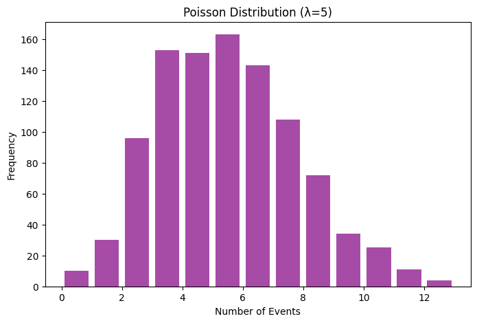

Geometric Distribution

The Geometric distribution is a discrete probability distribution that models the number of trials needed to achieve the first success in a sequence of independent Bernoulli trials, each with the same probability of success. It is a simple model that answers the question, “How many trials will it take to achieve the first success?”

Probability math representation:
The probability mass function (PMF) of the Geometric distribution for observing the first success on the $k$-th trial: $P(k|p) = (1-p)^{k-1}p$

where $p$ is the probability of success on a single trial, and $(1 - p)$ is the probability of failure.

Memoryless Property: The Geometric distribution has a unique memoryless property, meaning that the probability of success in future trials does not depend on the number of failures observed in the past.

Examples:

• The number of coin flips until the first head is observed.
• The number of sales calls needed until the first sale is made.

Python Example: In Python, you can simulate a Geometric distribution using numpy.random.geometric(p, size), where $p$ is the probability of success, and $size$ is the number of experiments.

p = 0.3  # Probability of success
size = 1000  # Number of samples
# Generating Geometric samples
geometric_samples = np.random.geometric(p, size)

# Plotting the distribution
plt.figure(figsize=(8, 5))
plt.hist(geometric_samples, bins=range(1, np.max(geometric_samples)+2), rwidth=0.8, color='orange', alpha=0.7)
plt.title('Geometric Distribution (p=0.3)')
plt.xlabel('Number of Trials Until First Success')
plt.ylabel('Frequency')
plt.show()

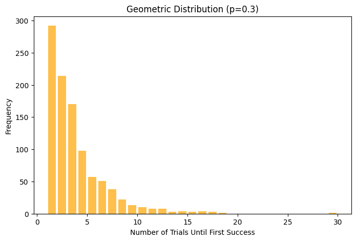
The distribution is skewed to the right, which is typical for Geometric distributions. This skewness indicates that while the first success might occur in the initial trials, there’s also a non-negligible probability of requiring a larger number of trials.

This kind of distribution is useful in scenarios where you’re interested in determining the likelihood of a certain number of attempts required to achieve a first success in repeated trials, such as the number of times a new task must be attempted before it is completed successfully.

Continuous Variables

Normal Distribution (Gaussian Distribution)

The Normal distribution, also known as the Gaussian distribution, is a continuous probability distribution that is symmetrical around its mean, showing that data near the mean are more frequent in occurrence than data far from the mean. It is one of the most important probability distributions in statistics due to its widespread occurrence in many natural phenomena.

Probability math representation:
The probability density function (PDF) of the Normal distribution is given by: $f(x | \mu, \sigma) = \frac{1}{\sigma \sqrt{2 \pi}} e^{ -\frac{1}{2} \left( \frac{x - \mu}{\sigma} \right)^2 }$

where $\mu$ is the mean or expectation of the distribution (also its median and mode), $\sigma$ is the standard deviation, $\sigma^2$ is the variance, $e$ is Euler’s number.

Characteristics:

• Symmetry: The Normal distribution is symmetric around its mean.
• Bell Curve: It has a bell-shaped curve where the spread of the distribution is determined by the standard deviation.
• Mean, Median, Mode: In a Normal distribution, the mean, median, and mode are all equal.
• Asymptotic: The tails of the distribution approach the x-axis asymptotically; theoretically, they never touch the x-axis.
• 68-95-99.7 Rule: About 68% of values drawn from a Normal distribution are within one standard deviation away from the mean; about 95% are within two standard deviations; and about 99.7% lie within three standard deviations.

Applications:

• In natural sciences and social sciences, the Normal distribution is used to represent real-valued random variables whose distributions are not known.
• In finance, it’s used to model asset prices, market returns, and various other financial variables.

Python Example:
In Python, you can use libraries like numpy and scipy to work with the Normal distribution. For example, numpy.random.normal(mu, sigma, size) can generate samples from a Normal distribution.

Let’s generate a sample from a Normal distribution with a mean of 0 and a standard deviation of 1, and plot the distribution.

mu = 0     # Mean
sigma = 1  # Standard deviation
size = 1000  # Number of samples

# Generating Normal distribution samples
normal_samples = np.random.normal(mu, sigma, size)

# Plotting the distribution
plt.figure(figsize=(8, 5))
plt.hist(normal_samples, bins=30, density=True, color='blue', alpha=0.7)
plt.title('Normal Distribution (μ=0, σ=1)')
plt.xlabel('Value')
plt.ylabel('Density')
plt.show()

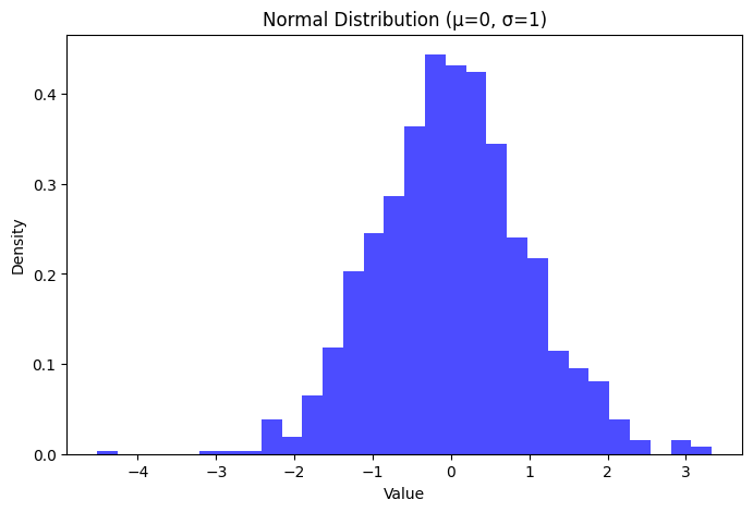
In this plot:

• The distribution forms the classic bell-shaped curve that is symmetric around the mean.
• Most of the data points are concentrated around the mean, with fewer points as you move further away.
• This particular Normal distribution, where $\mu$ = 0 and $\sigma$ = 1, is known as the Standard Normal Distribution.

The Normal distribution is fundamental in statistics and is often used as a first approximation to describe real-world variables that tend to cluster around a single mean value.

Uniform Distribution

The Uniform distribution, specifically the continuous uniform distribution, is a probability distribution where all outcomes are equally likely. Each interval of a given length within the distribution’s range has an equal probability of occurrence. It’s characterized by having a constant probability density function between its two bounds.

Probability math representation:
The probability density function (PDF) of the continuous uniform distribution between lower bound $a$ and upper bound $b$ is given by:

$f(x | a, b) = \begin{cases} \frac{1}{b - a} & \text{if } a \leq x \leq b, \\ 0 & \text{otherwise.} \end{cases}$

• The distribution is specified by these two parameters, $a$ and $b$, which define its range.

Mean and Median: The mean and median of a uniform distribution are ( \frac{a + b}{2} ).

Applications:

• Modeling equally likely outcomes, like the result of rolling a fair die (discrete case) or the error in a measurement that is uniformly distributed over a certain range.
• Random number generators often produce uniformly distributed “random” numbers.

Python Example:
A Uniform distribution can be simulated using numpy.random.uniform(a, b, size), where a is the lower bound, b is the upper bound, and size is the number of samples to generate.

Let’s generate a sample from a Uniform distribution with bounds $a = 0$ and $b = 1$, and plot the distribution.

# Reinitializing parameters for Uniform distribution
a = 0    # Lower bound
b = 1    # Upper bound
size = 1000  # Number of samples

# Generating Uniform distribution samples
uniform_samples = np.random.uniform(a, b, size)

# Plotting the distribution
plt.figure(figsize=(8, 5))
plt.hist(uniform_samples, bins=30, density=True, color='red', alpha=0.7)
plt.title('Uniform Distribution (a=0, b=1)')
plt.xlabel('Value')
plt.ylabel('Density')
plt.show()

In this plot:

• The distribution shows a constant probability density across the interval from 0 to 1.
• Each value within this range is equally likely to occur, as indicated by the uniform height of the bars across the entire range.
• The plot’s rectangular shape is characteristic of the continuous uniform distribution.

Exponential Distribution

The Exponential distribution is a continuous probability distribution that is commonly used to model the time or space between events in a Poisson process. It describes situations where events occur continuously and independently at a constant average rate.

Probability math representation:
The probability density function (PDF) of the Exponential distribution is given by:

$f(x | \lambda) = \lambda e^{-\lambda x}, for x \geq 0,$

where $\lambda$ is the rate parameter, and $e$ is Euler’s number (approximately 2.71828). The rate parameter $\lambda$ is the reciprocal of the mean. So, if events occur at an average rate of $\lambda$ per unit time, the mean time between events is $1/\lambda$.

Memoryless Property: The Exponential distribution is memoryless, which means that the probability of an event occurring in the next unit of time is independent of how much time has already elapsed.

Applications:

• Modeling the time until the next event in a Poisson process, such as the time until the next customer arrives at a service center.
• Estimating the lifespan of products and materials in reliability engineering.

Python Example: In Python, Exponential distributed data can be simulated using numpy.random.exponential(scale, size), where scale is the inverse of the rate parameter $\lambda$, and size is the number of samples.

Let’s generate a sample from an Exponential distribution with a mean time between events of 2 units (so, $\lambda = 0.5$), and plot the distribution.

# Parameters for Exponential distribution
scale = 2  # Scale parameter (inverse of lambda)
lambda_ = 1 / scale  # Rate parameter

# Generating Exponential distribution samples
exponential_samples = np.random.exponential(scale, size)

# Plotting the distribution
plt.figure(figsize=(8, 5))
plt.hist(exponential_samples, bins=30, density=True, color='brown', alpha=0.7)
plt.title('Exponential Distribution (λ=0.5)')
plt.xlabel('Time')
plt.ylabel('Density')
plt.show()

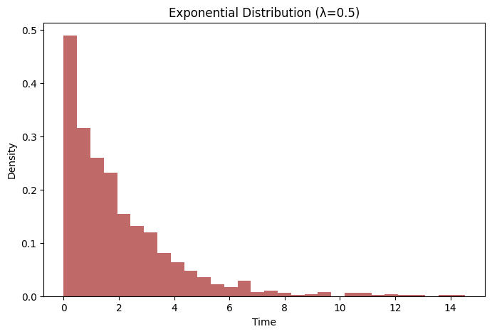
In this plot:

• The distribution shows a rapid decline from the left (near zero), demonstrating that shorter intervals between events are more likely.
• The curve is skewed to the right, which is characteristic of the Exponential distribution. This skewness indicates a long tail, meaning that while most events occur close to each other in time, there’s still a probability for events to occur with much longer intervals.
• The peak at the left end signifies the high probability of events occurring in a short interval, decreasing exponentially as the interval increases.

This type of distribution is particularly useful in modeling scenarios like the time until failure of mechanical components, the time between arrivals of customers at a service station, or any scenario where events happen continuously and independently at a constant average rate.

Beta Distribution

The Beta distribution is a family of continuous probability distributions defined on the interval [0, 1] parameterized by two positive shape parameters, denoted as $\alpha$ and $\beta$. It is particularly useful in modeling the behavior of random variables limited to intervals of finite length in a wide variety of disciplines including Bayesian analysis, finance, and economics.

Probability math representation:

• The probability density function (PDF) of the Beta distribution is given by: $f(x | \alpha, \beta) = \frac{x^{\alpha - 1}(1 - x)^{\beta - 1}}{B(\alpha, \beta)} for 0 \leq x \leq 1$,
  where $B(\alpha, \beta)$ is the beta function, which serves as a normalization constant to ensure the total probability is 1.

Characteristics:

• Flexibility in Shape: Depending on the values of $\alpha$ and $\beta$, the Beta distribution can take on different shapes including uniform, U-shaped, or J-shaped.
• Defined on [0, 1]: The Beta distribution is defined on the interval from 0 to 1, making it useful in modeling probabilities or proportions.
• Mean and Variance: The mean of the Beta distribution is $\frac{\alpha}{\alpha + \beta}$ and the variance is $\frac{\alpha \beta}{(\alpha + \beta)^2 (\alpha + \beta + 1)}$.

Applications:

• Bayesian Inference: Often used in Bayesian statistics, the Beta distribution is a conjugate prior distribution for binomial, Bernoulli, and geometric distributions.
• Modeling Proportions and Probabilities: For example, the Beta distribution can model the distribution of a probability of success in a process or an experiment.

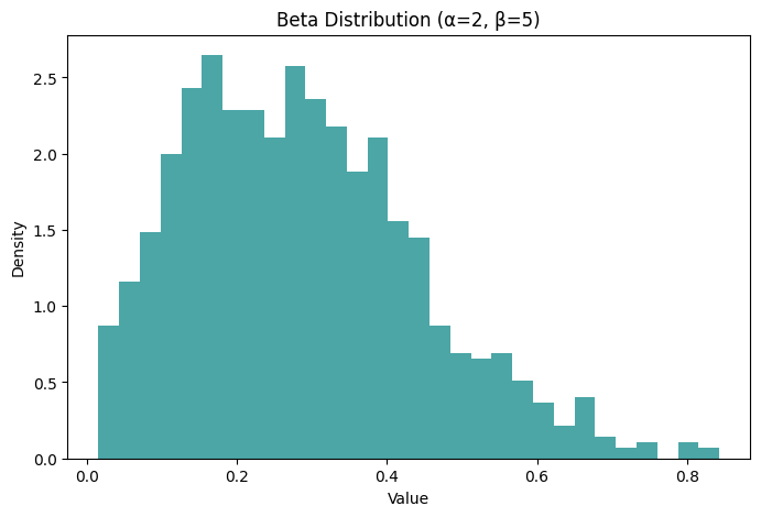
Python Example: In Python, you can use the scipy.stats.beta class to work with the Beta distribution. Let’s generate a sample from a Beta distribution with shape parameters $\alpha = 2$ and $\beta = 5$, and plot the distribution.

from scipy.stats import beta

# Parameters for Beta distribution
alpha = 2
beta_param = 5

# Generating Beta distribution samples
beta_samples = beta.rvs(alpha, beta_param, size=size)

# Plotting the distribution
plt.figure(figsize=(8, 5))
plt.hist(beta_samples, bins=30, density=True, color='teal', alpha=0.7)
plt.title('Beta Distribution (α=2, β=5)')
plt.xlabel('Value')
plt.ylabel('Density')
plt.show()

Here is the plot for the Beta distribution with shape parameters $\alpha = 2$ and $\beta = 5$, generated using 1000 samples.

In this plot:

• The distribution is skewed towards the left, indicating a higher probability density for lower values within the [0, 1] interval. This skewness is due to the relative values of $\alpha$ and $\beta$.
• The peak near the lower end of the range reflects the higher concentration of probability mass in that area.
• The shape of the Beta distribution in this case suggests that outcomes closer to 0 are more likely compared to those near 1.

The Beta distribution’s ability to assume various shapes makes it extremely versatile for modeling probabilities and proportions, especially in situations where the outcomes are constrained between 0 and 1, like in the case of proportions, rates, or probabilities in Bayesian analysis.

3. Specialized Distributions

Student’s t-Distribution

• Math Representation: ( f(t) = \frac{\Gamma((\nu+1)/2)}{\sqrt{\nu\pi},\Gamma(\nu/2)}\left(1+\frac{t^2}{\nu}\right)^{-(\nu+1)/2} )
• Generation Method: Derived as the distribution of the ratio of a standard normal variable and the square root of a scaled chi-squared variable.

Chi-Squared Distribution

• Math Representation: ( f(x|k) = \frac{1}{2^{k/2}\Gamma(k/2)}x^{k/2 - 1}e^{-x/2} )
• Generation Method: Generated by summing the squares of k independent standard normal random variables.

F-Distribution

• Math Representation: ( f(x|d_1, d_2) = \frac{\sqrt{\frac{(d_1x)^{d_1} \cdot d_2^{d_2}}{(d_1x+d_2)^{d_1+d_2}}}}{x \cdot B\left(\frac{d_1}{2}, \frac{d_2}{2}\right)} )
• Generation Method: Generated as the ratio of two scaled chi-squared distributed variables.

These distributions are foundational in statistics and are used based on the nature of the data (continuous, discrete) and the specific requirements of the analysis being conducted. Each distribution has unique properties and assumptions that make it suitable for different types of data and statistical inference needs.